Digital Feature: Relief valve sizing for two-phase flow

AUTHOR: Asutosh Chavda, Sarnia, Ontario, Canada

This article will present the sizing technique for two-phase flow through relief valves and orifices. The procedure is simple but rigorous and generally applicable.

The technique requires solving the Bernouli flow equation for mass flux density (lb/s/ft²). The point at which mass flux density is at a maximum corresponds to the choking pressure and flowrate. An important part of the technique in solving the flow equation is numerically integrating the density-pressure term, which is done by performing a series of constant entropy flash calculations from the pressure upstream of the nozzle to some downstream pressure. Data from the flashes are then used for numerical integration. After calculating the mass flux density, the area of the orifice or flowrate can be known if the other is known.

Two-phase relief flow occurs when mass of flow is a combination of a vapor and a liquid. Normally, two-phase relief is only considered for the device where two-phase flow enters the device or that two phase is produced as fluid moves through the relief device. API 520 has detailed scenarios that can be considered two-phase in Annexure C, Table C.1—professionals can consult the table for more reference. Two-phase relief requires 2x–10x more orifice area than single-phase relief would require.

API 520 describes two methods for solving two-phase flow: HEM and Omega. The HEM method assumes the fluid mixture behaves as a “pseudo-single-phase fluid” with a density that is the volume-averaged density of the two phases. The major postulate is that the fluid model is homogenous and at phase equillibrium, hence the acronym (HEM). Homogenous means the velocities (momentum flux) and temperature are at phase interface and the phases are also at equillibrium.

The Omega method was developed to avoid performing isentropic flashes and instead use a number of interpolations to achive the result. However, results have shown wide vairance and, as such, it is not a favored method for two-phase sizing. This article will not discuss the Omega method.

The following is a stepwise presentation of calculating the two-phase relief valve sizing technique described in API 520. The general energy balance for isentropic nozzle flow forms the basis of the Bernouli equation for the mass flux calculation, as presented in API 520.

For known throat pressure PT, the energy balance can be further simplied: 

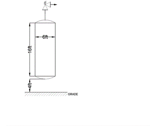
An example of two-phase calculation. This example is a vessel used as a treater and full with LPG liquid. The normal operating pressure is 80 psig and the maximum allowable working pressure (MAWP) of the vessel is 165 psig. The relief scenario that is considered is a fire case. API 521 states that two-phase relief device sizing is not normally required for the fire case, except for unusually foamy or reactive materials. However, it is worthwhile to ensure for certain systems that the area is not undersized for two-phase flow. To be on the conservative side, a normal vapor flow is calculated. Based on the relief load, an orifice is determined—it is advisable to then check for two-phase flow. For this article, a two-phase sizing is considered.

The vessel in this example is 6 ft in diameter and 16 ft T/T length with ellipsoidal heads. The standard heat absorption equation (as described in API 521) is used to calculate the vapor relief load.

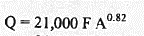
The heat input to the vessel can be calculated as per the API equation:

The heat absorbed in the vessel and latent heat of vaporization at the relieving condition can be used to calculate the mass relief rate. For this example, the mass relief load considered is 50,000 lb/hr. The heating path that is followed can be explained using the phase envelope.

Point 1: Initially, LPG is assumed to be subcooled and heat from the fire will cause the LPG to be heated. Constant volume expansion and pressurization of the liquid is happening at this point.

Point 2: The pressure increases to relieving pressure and only liquid relief is expected at this point.

Point 3: At this point, the LPG starts boiling and vapor generation will start.

Point 4: Two-phase relief begins (it will be mostly liquid). This is the sizing point for the two-phase flow.

Point 5: At this point, mostly vapor is releasing.

Calculation of mass flux. Using proprietary simulation software^a, a model is created for isentropic flashes (FIG. 1). An expander block is used with polytropic efficiency set at 100% for isentropic flashes. The pressure safety valve (PSV) inlet is the stream expected at the releif valve. A step-size pressure drop of 10 psi at each flash is arbitrarily selected, which is about 5% of relieving pressure.

FIG. 1. Isentropic flashes modeled in proprietary simulation software^a

Values for mixed-phase density and pressure from the proprietary software flashes are than tabulated in a spreadsheet to enable the calculation of mass flux at each pressure drop point, as shown in TABLE 1.

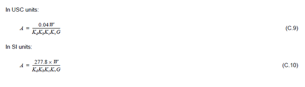
Finally, the orifice area of the relief valve is calculated using the following equation from API 520:

The coefficient of discharge in the equation above for chocked flow is taken for vapor, which is Kd=0.975. Based on the backpressure, Kb can be either 1 or for balance bellow can be read from the graph provided in API 520. For the above example the maximum flux value of 1784.15 lb/s*ft2 occurs at 160 Psig and requires 1.12 in2 of relief area. An Orifice “J,” having bore size of 1.287 in², is selected for the relief load.

NOTE

^a Aspen HYSYS

BIO

ASUTOSH CHAVDA has held different positions for Saudi Aramco, Bantral, Dubai Natural Gas Co. Ltd. and Fluor, among others. He has extensive experience in process design, FEED and detailed design, as well as experience in several different type of process technologies.

Related News

From the Archive

Comments

Comments

{{ error }}

Add Comment

{{ comment.name }} Editor • {{ comment.dateCreated | date:'short' }}

{{ comment.text }}